“In God we trust, the rest must come with data”
Narayan Murthy
This is a famous quote of Mr. Narayan Murthy, an Indian billionaire businessman. He is the co-founder of Infosys, and has been chairman, chief executive officer, president, and chief mentor, before retiring and taking the title chairman emeritus.
As apt as this seems on the first glance, upon deeper thought, one can’t help but realise that data can be manipulated to speak whatever we want it to. I’ve covered this in-depth on my other post here:
A Tale Of Numbers Versus Graphs
Data, of course, doesn’t lie but summary statistics most often does!
However, data is considered the new oil so we cannot just give up this easily. There has to be a way to make ourselves less prone to such basic inferencing errors. So, without much ado, lets dive straight into it.
1. DON’T IGNORE THE OBVIOUS: VISUALIZATION
Visualisation of extremely large datasets has never been easier. We, for example, have Python (seaborn library’s function called “pairplot”), MATLAB, R, and many more such tools at our disposal. There are tons of pre-existing functions which enables us to plot the dataset in different ways graphing formats and styles.
However, with more tools, comes the problem of plenty! You can plot the distribution of each variable individually or examine their cross-relations.
Tip: Do not plot more than 3 variables against each other unless you are a super-human. Know your strengths and limitations!
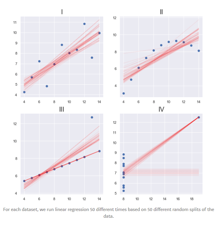
2. CROSS-VALIDATION AND HOLD-OUT SETS
This goes a bit into machine learning. If you’re new to this, here’s a gist of what it does:
In machine learning, we feed the computer with a list of pairwise inputs and outputs. The computer tries to find an equation which fits all the datasets as well as possible. This is called as training our model. Once this is done, the model can be used to make predictions about the output a given input is most likely to generate. Under cross-validation and hold-out sets, we use only a subset of the list of pairwise input-outputs to train our model and then test it on another subset from the same list to check its accuracy.
Residuals is a measure of how far away from the regression line the data points are. In simpler terms, the difference between predicted and actual value of the output. Root Mean Square Error (RSME) is the square root of the residuals ie. Prediction errors. Applying this on Anscombe’s Quartet, we get:
| DATASET | RSME (approx. using 3-fold cross-validation) |
| Dataset I | 1.3 |
| Dataset II | 1.3 |
| Dataset III | 1.5 |
| Dataset IV | 1.9 |
We can already see the differences starting to show.
If we want to dive deeper, we can calculate the confidence intervals and p-values for the linear model coefficients.
Python’s scikit-learn’s cross_val_score function and LinearRegression class will come in handy here if you want to implement this. For plotting, use matplotlib’s plt.subplots() function.
3. OTHER STATISTICAL MEASURES:
Statistics is much wider and deeper than just the mean, variance, and correlation. It is not the aim of this post to delve deeper into statistics but here are some terms which you might want to look into to analyse any dataset before making inferences. It includes, but is not limited to, the following:
- Skewness
- Kurtosis
- Jarque-Bera
- Autocorrelation
- Non-linearity
- Heteroscedasticity
Python’s statsmodels’ Ordinary Least Squares (OLS) class will help us get access to some of these stats. Just use the .summary() function.
I’ll be sharing a detailed coding for the concepts above so keep an eye out 🙂
